The synoptic "big picture" for the area around San Antonio, Texas for February 2, 2007 predicted that the air mass over the area would begin the period quite dry as shown below on the 30 hor forecast from the February 1, 2007 0Z AVN model output. Looking at the lower left panel you can see that the relative humidity over Texas is extremely low in the range of less than 30% at 700mb. Clicking on the image below will open up an aminated sequence that runs from 30 through 54 hours, or from midnight February 2nd, the beginning of the forecast period, through midnight Saturday morning, February 3rd the end of our forecast period. As you can see in the animation the entire period is characterized by quite dry air over the region. For comparison you can also look at the AVN model from 12Z on February 2, 2007 as well as the WRF model from 0Z on February 1st and 12Z on February 1, 2007. Looking at these other sequences you can see a similar prediction for a very dry air mass over the region and in looking at the lower right panels on each, you also see that the area is not expecting any precipitation during the period either.

(February 1, 2007 0Z AVN model output at 30 hours valid at 06Z February 2, 2007 Courtesy of the Pennsylvania State University e-Wall showing the extremely dry air over the Texas area - Click image for 30-54 hour animation sequence)

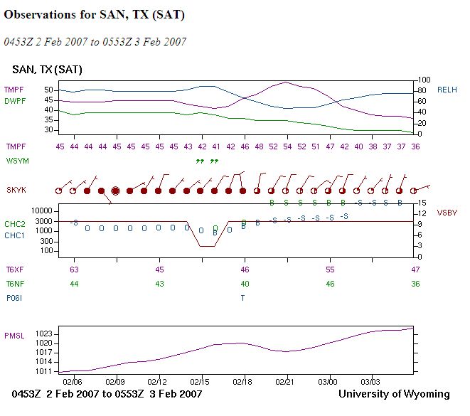
In the process of making the forecast, I also looked at the results of the February 3rd 12Z output of model output statistics, or MOS from three different forecasting models, the NGM, the ETA and the GFS as well as the output from the 18Z GFS model. To see detailed information from these models please click this link. In looking at these various forecast models I computed the average of their various high and low predictions which came out to a high of 68 and a low of 43 degrees. For my forecast since the 18Z GFS MOS output was somewhat cooler than the 12Z GFS run, I chose to lower my high temperature forecast just slightly and predicted a high of 67 and a low of 43 degrees.

The actual high and low temperatures (click link for a copy of the Weather Challenge results) where quite different than what I had forecast with a high of just 55 and a low of 36 degrees, both far below what I had expected to occur.

So what went wrong with the forecast and what will I do differently in the future?

Looking at the meteogram for San Antonio, Texas for the forecast period (shown below), we can see that rather than the expected clear skies through the period as predicted by the various forecast models above, we in fact had a mostly cloudy day (shown by the mostly filled in red circles from 7Z through 19Z) that then turned clear in the evening (indicated by the mostly white circles from 19Z through the end of the period on the right). Winds were also lighter than expected, especially in the evening hours, as shown by the short barbs in the last 5 wind indictions from the red circles in the second row from the right. As a result of the persistent cloud cover during the daytime hours over the area far less incoming solar radiation was received and as a result the temperature did not warm up nearly as much as expected or forecast. Likewise, the clearing skies and light winds in the evening hours resulted in a much larger than anticipated radiational cooling of the area and as a result the temperature dropped rapidly as shown by the upper graph purple trace where you can see the temperature falls from 47F at 6pm (0Z) to 36 by midnight (6Z), a drop of 11 degrees in just 6 hours.

(February 3, 2007 San Antonio, Texas meteogram showing the persistence of clouds and late clearing which resulted in the lower than expected temperatures. Meteogram courtesy of the University of Wyoming)

So as a result of this, what lessons were learned here? In my opinion, had I taken a more careful look at the numerical model loops that I showed in the first portion of this analysis and not based my forecast almost exclusively on the MOS output and its consensus, I may have caught on to the fact that the winds were going to be far lighter than forecast by MOS,  and that given the low humidities, especially late in the period, I may have picked up on the fact that the area was in for a rapid, dramatic cool down in the evening hours under clear skies and light winds. Clearly, basing a forecast on just one or two tools or items of information is not sound forecasting practice, and in the future I need to be conscious of this fact and attempt to actively include more than just the easily obtained and used MOS outputs to make a forecast. Instead I need to look at not only the MOS outputs but the other numerical models, which can easily give far more information than a simple text output from MOS does.

Main Page Previous 1  2  3  5  6  Next